Voltage Response of a Low Pass Filter Applied to a Square Wave
A common technique to generate an adjustable fixed voltage from a microcontroller is to low pass filter a pulse width modulated signal. It's common knowledge that a rough estimate of the generated voltage will be . Here, I will prove this approximation correct and also derive other interesting properties of the resulting voltage, like the rate at which the transient response dies out, and an equivalent approximation in the case that the charging and discharging resistors are unequal. In fact, this case is a generalization of the single resistor case, so let's consider the double resistor case first.
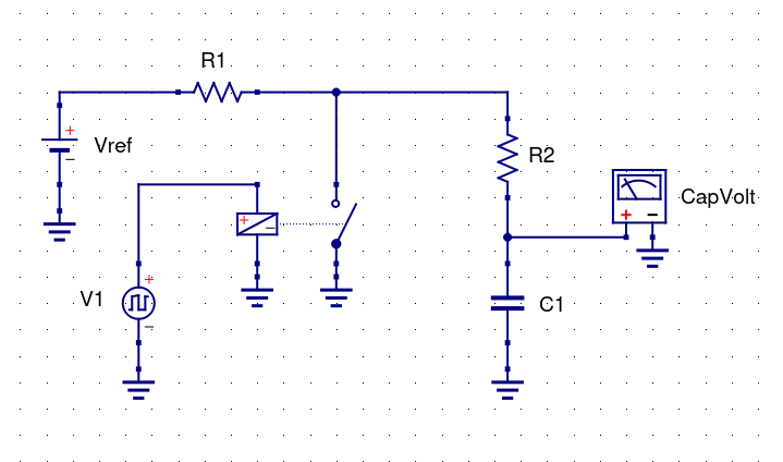
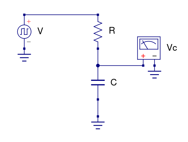
Figure 1. Square wave generated by a voltage reference. A relais is used as a model of a perfect transistor.Figure 2. Single resistor, or case of figure 1.
Let's say the capacitor voltage is right after the nth high pulse. During the next low pulse the voltage will drop exponentially with time constant . So right after the low pulse the capacitor voltage is:
Subsequently the input voltage will go high again, and this time the difference between the driving voltage and the capacitor voltage will drop off exponentially with the time constant .
Substituting we have now found a recurrence relation for the capacitor voltage after every high voltage pulse. To simplify further analysis we introduce the time independent variables and .
We now try to solve this recurrence relation. Starting with a uncharged capacitor we calculate the first few voltages.
This seems just to be a geometric series. For which we know the general formula.
Now is an exponential function with a negative exponent, so . The transient response will die out, and we can find the steady state capacitor voltage as.
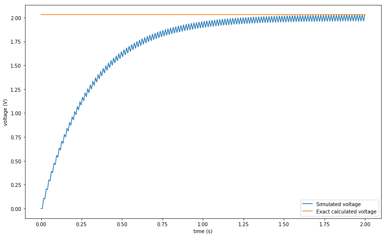
Figure 3. For the simulated voltage the values , , , were used. The horizontal line is the voltage given by the expression immediately preceding the figure.
This is as far as we can go in the general case. But if we use a high frequency signal the pulse times and will be very small which invites a taylor expansion.
Working this out gives:
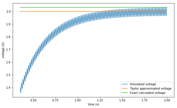
Figure 4. The simulated voltage from figure 1 is repeated here on a different time scale. The Taylor approximated voltage is given by the expression immediately preceding the figure.
If we now write for a suitable constant we find
Going back to the the one resistor case we recover the familiar rule of thumb.